Numpy, Pandas, Matplotlib#
Numpy
Pandas
Matplotlib
Seaborn
Numpy#
Numpy е библиотека създадена за работа с масиви. Масивите са едномерни, двумерни и т.н. Масивите са еднотипни, т.е. всички елементи в масива трябва да са от един и същи тип. Масивите са с фиксиран размер, т.е. не може да се добавят или премахват елементи от масива. Масивите са с фиксиран тип, т.е. всички елементи в масива трябва да са от един и същи тип. Масивите са с фиксиран размер, т.е. не може да се добавят или премахват елементи от масива.
!pip install numpy
Requirement already satisfied: numpy in /home/lyubolp/.local/lib/python3.8/site-packages (1.24.1)
Едни от важните характеристики на масивите са:
shape - размер на масива
dtype - тип на елементите в масива
ndim - брой измерения на масива
size - общ брой елементи в масива
def display_numpy_array_info(arr):
    print(f'{arr=}')
    print(f'{arr.shape=}')
    print(f'{arr.dtype=}')
    print(f'{arr.ndim=}')
    print(f'{arr.size=}')
    print('')
Можем да създадем масив от списък, с помощта на функцията array.
import numpy as np

arr = np.array([[1, 2, 3, 4, 5], [6, 7, 8, 9, 10]])

display_numpy_array_info(arr)
arr=array([[ 1,  2,  3,  4,  5],
       [ 6,  7,  8,  9, 10]])
arr.shape=(2, 5)
arr.dtype=dtype('int64')
arr.ndim=2
arr.size=10
Можем да зададем типа на елементите в масива с помощта на параметъра dtype.
import numpy as np

arr = np.array([1.1, 2.2, 3.3, 4.4, 5.5], dtype=np.float32)

display_numpy_array_info(arr)
arr=array([1.1, 2.2, 3.3, 4.4, 5.5], dtype=float32)
arr.shape=(5,)
arr.dtype=dtype('float32')
arr.ndim=1
arr.size=5
С помощта на функцията arange можем да създадем масив с равномерни елементи от start до end със стъпка step.
import numpy as np

arr1 = np.arange(1, 10, 2)
arr2 = np.arange(2, 10, 1)

display_numpy_array_info(arr1)
display_numpy_array_info(arr2)
arr=array([1, 3, 5, 7, 9])
arr.shape=(5,)
arr.dtype=dtype('int64')
arr.ndim=1
arr.size=5

arr=array([2, 3, 4, 5, 6, 7, 8, 9])
arr.shape=(8,)
arr.dtype=dtype('int64')
arr.ndim=1
arr.size=8
Можем да създадем масив от нули или единици, с помощта на функциите zeros и ones.
import numpy as np

zeros = np.zeros((3, 4))
ones = np.ones((2, 3, 4), dtype=np.int16)

display_numpy_array_info(zeros)
display_numpy_array_info(ones)
arr=array([[0., 0., 0., 0.],
       [0., 0., 0., 0.],
       [0., 0., 0., 0.]])
arr.shape=(3, 4)
arr.dtype=dtype('float64')
arr.ndim=2
arr.size=12

arr=array([[[1, 1, 1, 1],
        [1, 1, 1, 1],
        [1, 1, 1, 1]],

       [[1, 1, 1, 1],
        [1, 1, 1, 1],
        [1, 1, 1, 1]]], dtype=int16)
arr.shape=(2, 3, 4)
arr.dtype=dtype('int16')
arr.ndim=3
arr.size=24
С метода random можем да създадем масив със случайни числа в интервала от 0 до 1 с размери rows и cols.
import numpy as np

random = np.random.random((2, 3))

display_numpy_array_info(random)
arr=array([[0.85258647, 0.87437575, 0.04258029],
       [0.06627148, 0.24665089, 0.52177255]])
arr.shape=(2, 3)
arr.dtype=dtype('float64')
arr.ndim=2
arr.size=6
С метода reshape можем да преоразмерим масива.
import numpy as np

arr = np.array([[1, 2, 3], [4, 5, 6]])
display_numpy_array_info(arr)

arr1 = arr.reshape(3, 2)
display_numpy_array_info(arr1)
arr=array([[1, 2, 3],
       [4, 5, 6]])
arr.shape=(2, 3)
arr.dtype=dtype('int64')
arr.ndim=2
arr.size=6

arr=array([[1, 2],
       [3, 4],
       [5, 6]])
arr.shape=(3, 2)
arr.dtype=dtype('int64')
arr.ndim=2
arr.size=6
Numpy поддържа и някои математически операции между масиви.
import numpy as np

a = np.array([10, 20, 30])
b = np.array([5, 7, 8])

print(a + b)
print(a - b)
print(a * b)
print(a / b)
print(a ** 2)
print(a / 10)
print(a > 15)
[15 27 38]
[ 5 13 22]
[ 50 140 240]
[2.         2.85714286 3.75      ]
[100 400 900]
[1. 2. 3.]
[False  True  True]
import numpy as np

a = np.random.random((2, 3)) * 100

print(a)
print(a.sum())
print(a.min())
print(a.max())
print(a.std())
[[71.34135627  0.25907481 89.56057185]
 [94.61009345 24.91787537 77.29307812]]
357.98204987140775
0.2590748147073829
94.61009345054515
34.87696903183212
import numpy as np

b = np.arange(1, 10)
print(b)
print(np.exp(b))
print(np.sqrt(b))
[1 2 3 4 5 6 7 8 9]
[2.71828183e+00 7.38905610e+00 2.00855369e+01 5.45981500e+01
 1.48413159e+02 4.03428793e+02 1.09663316e+03 2.98095799e+03
 8.10308393e+03]
[1.         1.41421356 1.73205081 2.         2.23606798 2.44948974
 2.64575131 2.82842712 3.        ]
Numpy поддържа и сумиране на масиви, по даден ред или колона.
import numpy as np

c = np.array([[1, 2, 3], [4, 5, 6]])
print(c)
print(c.sum(axis=0))
print(c.sum(axis=1))
[[1 2 3]
 [4 5 6]]
[5 7 9]
[ 6 15]
Една особеност на Numpy е индексацията. Ако имаме двумерен масив, и искаме да достъпим елемента на 0-лев ред и 1-ви колона, то индексацията е следната arr[0, 1]. Ако използваме само един индекс, то той се отнася за редовете. Т.е. arr[0] ще ни върне първия ред от масива. Ако искаме да изберем цял ред, колона или която и да е друга размерност, можем да използваме :. Т.е. arr[:, 1] ще ни върне всички редове от втората колона.
import numpy as np

a = np.arange(1, 13).reshape(3, 4)

print(a)

print(f'{a[0, 1]=}')
print(f'{a[1, :]=}')
print(f'{a[:, 2]=}')

a[0, 1] = 1
print(a)
[[ 1  2  3  4]
 [ 5  6  7  8]
 [ 9 10 11 12]]
a[0, 1]=2
a[1, :]=array([5, 6, 7, 8])
a[:, 2]=array([ 3,  7, 11])
[[ 1  1  3  4]
 [ 5  6  7  8]
 [ 9 10 11 12]]
Освен с числа, можем да индексираме и с булеви масиви. Можем да подадем масив от булеви стойности - ако стойността на даден елемент е True, то той ще бъде включен в резултата, а ако е False, то няма да бъде включен.
import numpy as np

a = np.arange(1, 10)
print(a)

even_mask = a % 2 == 0
print(a[even_mask])
print(a[a % 2 == 0])
[1 2 3 4 5 6 7 8 9]
[2 4 6 8]
[2 4 6 8]
Numpy поддържа три вида копиране - никакво, плитко и дълбоко.
Когато извикаме arr2 = arr1, то това е никакво копиране. Т.е. arr2 е просто друго име на arr1. Ако променим елемента на arr2, то той ще се промени и в arr1.
Когато извикаме arr3 = arr.view(), ще се създаде нов обект, но данните няма да се копират.
Когато извикаме arr4 = arr.copy(), ще се създаде нов обект, с копие на данните.
import numpy as np

a = np.arange(1, 13).reshape(3, 4)
print(a)

b = a
c = a.view()
d = a.copy()

a[0, 0] = 100

print(b)
print(c)
print(d)

print(b is a)
print(c is a)
print(d is a)
[[ 1  2  3  4]
 [ 5  6  7  8]
 [ 9 10 11 12]]
[[100   2   3   4]
 [  5   6   7   8]
 [  9  10  11  12]]
[[100   2   3   4]
 [  5   6   7   8]
 [  9  10  11  12]]
[[ 1  2  3  4]
 [ 5  6  7  8]
 [ 9 10 11 12]]
True
False
False
Numpy ни позволява да прилагаме функции към нашите масиви. Например, можем да приложим функцията sqrt към всеки елемент на масива.
import numpy as np

def square(x):
    return x ** 2

a = np.arange(1, 10)

print(a)

b = square(a)
display_numpy_array_info(b)
[1 2 3 4 5 6 7 8 9]
arr=array([ 1,  4,  9, 16, 25, 36, 49, 64, 81])
arr.shape=(9,)
arr.dtype=dtype('int64')
arr.ndim=1
arr.size=9
Pandas#
Pandas е библиотека, която ни позволява да работим с таблични данни. Поддържа множество формати за входни данни - csv, json, html, excel, sql и др.
!pip install pandas
Collecting pandas
  Using cached pandas-1.5.2-cp38-cp38-manylinux_2_17_x86_64.manylinux2014_x86_64.whl (12.2 MB)
Requirement already satisfied: python-dateutil>=2.8.1 in /home/lyubolp/.local/lib/python3.8/site-packages (from pandas) (2.8.2)
Collecting pytz>=2020.1
  Downloading pytz-2022.7.1-py2.py3-none-any.whl (499 kB)
     |████████████████████████████████| 499 kB 2.2 MB/s eta 0:00:01
?25hRequirement already satisfied: numpy>=1.20.3; python_version < "3.10" in /home/lyubolp/.local/lib/python3.8/site-packages (from pandas) (1.24.1)
Requirement already satisfied: six>=1.5 in /usr/lib/python3/dist-packages (from python-dateutil>=2.8.1->pandas) (1.14.0)
Installing collected packages: pytz, pandas
Successfully installed pandas-1.5.2 pytz-2022.7.1
Pandas поддържа 3 вида структури - Series, DataFrame и Panel
Series- едномерен масивDataFrame- двумерна таблицаPanel- тримерна структура
Series#
import pandas as pd

a = pd.Series([10, 20, 30, 40, 50])
b = pd.Series([1.1, 2.2, 3.3, 4.4, 5.5], dtype=np.float32)

print(a)
print(b)
0    10
1    20
2    30
3    40
4    50
dtype: int64
0    1.1
1    2.2
2    3.3
3    4.4
4    5.5
dtype: float32
import pandas as pd

a = pd.Series([10, 20, 30, 40, 50], index=['a', 'b', 'c', 'd', 'e'])
b = pd.Series({'a': 10, 'b': 20, 'c': 30, 'd': 40, 'e': 50})

print(a)
print(b)
a    10
b    20
c    30
d    40
e    50
dtype: int64
a    10
b    20
c    30
d    40
e    50
dtype: int64
import pandas as pd

a = pd.Series([10, 20, 30, 40, 50], index=['a', 'b', 'c', 'd', 'e'])


print(a[0])
print(a['b'])
print(a[1:4])
10
20
b    20
c    30
d    40
dtype: int64
import pandas as pd

a = pd.Series([10, 20, 30, 40, 50])
b = pd.Series([1, 2, 3, 4, 5])

print(a + b)
print(a - b)
print(a * b)
print(a / b)
0    11
1    22
2    33
3    44
4    55
dtype: int64
0     9
1    18
2    27
3    36
4    45
dtype: int64
0     10
1     40
2     90
3    160
4    250
dtype: int64
0    10.0
1    10.0
2    10.0
3    10.0
4    10.0
dtype: float64
import pandas as pd

a = pd.Series([10, 20, 30, 40, 50])

print(a.sum())
print(a.max())
print(a.min())
150
50
10
DataFrame#
import pandas as pd

data = [1, 2, 3, 4, 5]
df = pd.DataFrame(data)

df
| 0 | |
|---|---|
| 0 | 1 |
| 1 | 2 |
| 2 | 3 |
| 3 | 4 |
| 4 | 5 |
import pandas as pd

data = [['Alex', 20], ['Bob', 22], ['Clarke', 23]]
df = pd.DataFrame(data, columns=['Name', 'Age'])

df
| Name | Age | |
|---|---|---|
| 0 | Alex | 20 |
| 1 | Bob | 22 |
| 2 | Clarke | 23 |
import pandas as pd

df = pd.DataFrame({'Name': ['Alex', 'Bob', 'Clarke'], 'Age': [20, 22, 23]})

df
| Name | Age | |
|---|---|---|
| 0 | Alex | 20 |
| 1 | Bob | 22 |
| 2 | Clarke | 23 |
import pandas as pd

df = pd.DataFrame({'Name': ['Alex', 'Bob', 'Clarke'], 'Age': [20, 22, 23]})

df['Name']
0      Alex
1       Bob
2    Clarke
Name: Name, dtype: object
import pandas as pd

df = pd.DataFrame({
    'Name': ['Alex', 'Bob', 'Clarke', 'Nathan', 'Johny'],
    'Age': [20, 22, 23, 19, 21],
    'Height': [170, 180, 175, 165, 172]
    })

df.loc[:2]
| Name | Age | Height | |
|---|---|---|---|
| 0 | Alex | 20 | 170 |
| 1 | Bob | 22 | 180 |
| 2 | Clarke | 23 | 175 |
import pandas as pd

df = pd.DataFrame({
    'Name': ['Alex', 'Bob', 'Clarke', 'Nathan', 'Johny'],
    'Age': [20, 22, 23, 19, 21],
    'Height': [170, 180, 175, 165, 172]
    })

df.loc[1]
Name      Bob
Age        22
Height    180
Name: 1, dtype: object
import pandas as pd

df = pd.DataFrame({
    'Name': ['Alex', 'Bob', 'Clarke', 'Nathan', 'Johny'],
    'Age': [20, 22, 23, 19, 21],
    'Height': [170, 180, 175, 165, 172]
    })

df.iloc[1]
Name      Bob
Age        22
Height    180
Name: 1, dtype: object
import pandas as pd

df = pd.DataFrame({
    'Name': ['Alex', 'Bob', 'Clarke', 'Nathan', 'Johny', 'Bobby', 'Roger', 'Tom', 'Jerry', 'Mickey'],
    'Age': [20, 22, 23, 19, 21, 20, 22, 23, 19, 21],
    'Height': [170, 180, 175, 165, 172, 170, 180, 175, 165, 172]
    })

df.head()
| Name | Age | Height | |
|---|---|---|---|
| 0 | Alex | 20 | 170 |
| 1 | Bob | 22 | 180 |
| 2 | Clarke | 23 | 175 |
| 3 | Nathan | 19 | 165 |
| 4 | Johny | 21 | 172 |
import pandas as pd

df = pd.DataFrame({
    'Name': ['Alex', 'Bob', 'Clarke', 'Nathan', 'Johny', 'Bobby', 'Roger', 'Tom', 'Jerry', 'Mickey'],
    'Age': [20, 22, 23, 19, 21, 20, 22, 23, 19, 21],
    'Height': [170, 180, 175, 165, 172, 170, 180, 175, 165, 172]
    })

df.tail()
| Name | Age | Height | |
|---|---|---|---|
| 5 | Bobby | 20 | 170 |
| 6 | Roger | 22 | 180 |
| 7 | Tom | 23 | 175 |
| 8 | Jerry | 19 | 165 |
| 9 | Mickey | 21 | 172 |
import pandas as pd

df = pd.DataFrame({
    'Name': ['Alex', 'Bob', 'Clarke', 'Nathan', 'Johny', 'Bobby', 'Roger', 'Tom', 'Jerry', 'Mickey'],
    'Age': [20, 22, 23, 19, 21, 20, 22, 23, 19, 21],
    'Height': [170, 180, 175, 165, 172, 170, 180, 175, 165, 172]
    })

df.describe()
| Age | Height | |
|---|---|---|
| count | 10.000000 | 10.000000 |
| mean | 21.000000 | 172.400000 |
| std | 1.490712 | 5.274677 |
| min | 19.000000 | 165.000000 |
| 25% | 20.000000 | 170.000000 |
| 50% | 21.000000 | 172.000000 |
| 75% | 22.000000 | 175.000000 |
| max | 23.000000 | 180.000000 |
import pandas as pd

df = pd.DataFrame({
    'Name': ['Alex', 'Bob', 'Clarke', 'Nathan', 'Johny', 'Bobby', 'Roger', 'Tom', 'Jerry', 'Mickey'],
    'Age': [20, 22, 23, 19, 21, 20, 22, 23, 19, 21],
    'Height': [170, 180, 175, 165, 172, 170, 180, 175, 165, 172]
    })

df[['Age', 'Height']].groupby('Age').mean()
| Height | |
|---|---|
| Age | |
| 19 | 165.0 |
| 20 | 170.0 |
| 21 | 172.0 |
| 22 | 180.0 |
| 23 | 175.0 |
import pandas as pd

df = pd.DataFrame({
    'Name': ['Alex', 'Bob', 'Clarke', 'Nathan', 'Johny', 'Bobby', 'Roger', 'Tom', 'Jerry', 'Mickey'],
    'Age': [20, 22, 23, 19, 21, 20, 22, 23, 19, 21],
    'Height': [170, 180, 175, 165, 172, 170, 180, 175, 165, 172]
    })

df[['Age', 'Height']].groupby('Age').count()
| Height | |
|---|---|
| Age | |
| 19 | 2 |
| 20 | 2 |
| 21 | 2 |
| 22 | 2 |
| 23 | 2 |
import pandas as pd
import os

df = pd.read_csv(os.path.join('titanic', 'train.csv'))

df.head()
| PassengerId | Survived | Pclass | Name | Sex | Age | SibSp | Parch | Ticket | Fare | Cabin | Embarked | |
|---|---|---|---|---|---|---|---|---|---|---|---|---|
| 0 | 1 | 0 | 3 | Braund, Mr. Owen Harris | male | 22.0 | 1 | 0 | A/5 21171 | 7.2500 | NaN | S |
| 1 | 2 | 1 | 1 | Cumings, Mrs. John Bradley (Florence Briggs Th... | female | 38.0 | 1 | 0 | PC 17599 | 71.2833 | C85 | C |
| 2 | 3 | 1 | 3 | Heikkinen, Miss. Laina | female | 26.0 | 0 | 0 | STON/O2. 3101282 | 7.9250 | NaN | S |
| 3 | 4 | 1 | 1 | Futrelle, Mrs. Jacques Heath (Lily May Peel) | female | 35.0 | 1 | 0 | 113803 | 53.1000 | C123 | S |
| 4 | 5 | 0 | 3 | Allen, Mr. William Henry | male | 35.0 | 0 | 0 | 373450 | 8.0500 | NaN | S |
import pandas as pd
import os

df = pd.DataFrame({
    'Name': ['Alex', 'Bob', 'Clarke', 'Nathan', 'Johny', 'Bobby', 'Roger', 'Tom', 'Jerry', 'Mickey'],
    'Age': [20, 22, 23, 19, 21, 20, 22, 23, 19, 21],
    'Height': [170, 180, 175, 165, 172, 170, 180, 175, 165, 172]
    })

df.to_csv('people.csv')
!cat people.csv
,Name,Age,Height
0,Alex,20,170
1,Bob,22,180
2,Clarke,23,175
3,Nathan,19,165
4,Johny,21,172
5,Bobby,20,170
6,Roger,22,180
7,Tom,23,175
8,Jerry,19,165
9,Mickey,21,172
Matplotlib#
!pip install matplotlib
Collecting matplotlib
  Downloading matplotlib-3.6.3-cp38-cp38-manylinux_2_12_x86_64.manylinux2010_x86_64.whl (9.4 MB)
     |████████████████████████████████| 9.4 MB 7.1 MB/s eta 0:00:01
?25hCollecting pyparsing>=2.2.1
  Downloading pyparsing-3.0.9-py3-none-any.whl (98 kB)
     |████████████████████████████████| 98 kB 4.7 MB/s  eta 0:00:01
?25hRequirement already satisfied: packaging>=20.0 in /home/lyubolp/.local/lib/python3.8/site-packages (from matplotlib) (22.0)
Collecting contourpy>=1.0.1
  Downloading contourpy-1.0.7-cp38-cp38-manylinux_2_17_x86_64.manylinux2014_x86_64.whl (300 kB)
     |████████████████████████████████| 300 kB 8.1 MB/s eta 0:00:01
?25hRequirement already satisfied: python-dateutil>=2.7 in /home/lyubolp/.local/lib/python3.8/site-packages (from matplotlib) (2.8.2)
Collecting pillow>=6.2.0
  Downloading Pillow-9.4.0-cp38-cp38-manylinux_2_17_x86_64.manylinux2014_x86_64.whl (3.3 MB)
     |████████████████████████████████| 3.3 MB 5.5 MB/s eta 0:00:01
?25hCollecting fonttools>=4.22.0
  Downloading fonttools-4.38.0-py3-none-any.whl (965 kB)
     |████████████████████████████████| 965 kB 7.8 MB/s eta 0:00:01
?25hRequirement already satisfied: numpy>=1.19 in /home/lyubolp/.local/lib/python3.8/site-packages (from matplotlib) (1.24.1)
Collecting cycler>=0.10
  Downloading cycler-0.11.0-py3-none-any.whl (6.4 kB)
Collecting kiwisolver>=1.0.1
  Downloading kiwisolver-1.4.4-cp38-cp38-manylinux_2_5_x86_64.manylinux1_x86_64.whl (1.2 MB)
     |████████████████████████████████| 1.2 MB 5.4 MB/s eta 0:00:01
?25hRequirement already satisfied: six>=1.5 in /usr/lib/python3/dist-packages (from python-dateutil>=2.7->matplotlib) (1.14.0)
Installing collected packages: pyparsing, contourpy, pillow, fonttools, cycler, kiwisolver, matplotlib
  WARNING: The scripts fonttools, pyftmerge, pyftsubset and ttx are installed in '/home/lyubolp/.local/bin' which is not on PATH.
  Consider adding this directory to PATH or, if you prefer to suppress this warning, use --no-warn-script-location.
Successfully installed contourpy-1.0.7 cycler-0.11.0 fonttools-4.38.0 kiwisolver-1.4.4 matplotlib-3.6.3 pillow-9.4.0 pyparsing-3.0.9
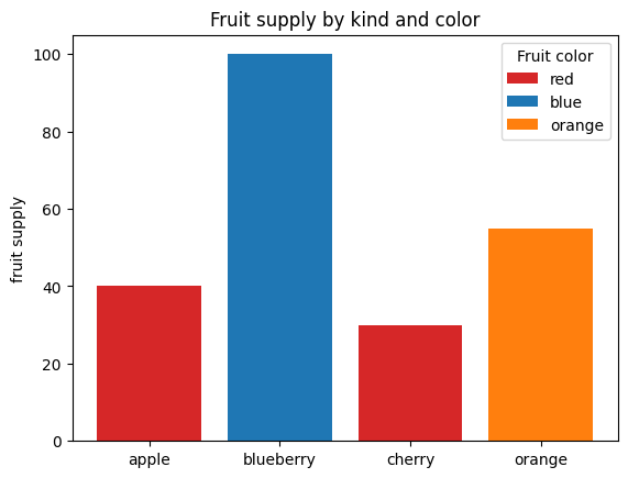
import matplotlib.pyplot as plt

fig, ax = plt.subplots()

fruits = ['apple', 'blueberry', 'cherry', 'orange']
counts = [40, 100, 30, 55]
bar_labels = ['red', 'blue', '_red', 'orange']
bar_colors = ['tab:red', 'tab:blue', 'tab:red', 'tab:orange']

ax.bar(fruits, counts, label=bar_labels, color=bar_colors)

ax.set_ylabel('fruit supply')
ax.set_title('Fruit supply by kind and color')
ax.legend(title='Fruit color')

plt.show()
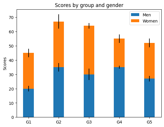
import matplotlib.pyplot as plt


labels = ['G1', 'G2', 'G3', 'G4', 'G5']
men_means = [20, 35, 30, 35, 27]
women_means = [25, 32, 34, 20, 25]
men_std = [2, 3, 4, 1, 2]
women_std = [3, 5, 2, 3, 3]
width = 0.35       # the width of the bars: can also be len(x) sequence

fig, ax = plt.subplots()

ax.bar(labels, men_means, width, yerr=men_std, label='Men')
ax.bar(labels, women_means, width, yerr=women_std, bottom=men_means,
       label='Women')

ax.set_ylabel('Scores')
ax.set_title('Scores by group and gender')
ax.legend()

plt.show()
import numpy as np
import matplotlib.pyplot as plt

# Fixing random state for reproducibility
np.random.seed(19680801)

dt = 0.01
t = np.arange(0, 30, dt)
nse1 = np.random.randn(len(t))                 # white noise 1
nse2 = np.random.randn(len(t))                 # white noise 2

# Two signals with a coherent part at 10 Hz and a random part
s1 = np.sin(2 * np.pi * 10 * t) + nse1
s2 = np.sin(2 * np.pi * 10 * t) + nse2

fig, axs = plt.subplots(2, 1)
axs[0].plot(t, s1, t, s2)
axs[0].set_xlim(0, 2)
axs[0].set_xlabel('Time')
axs[0].set_ylabel('s1 and s2')
axs[0].grid(True)

cxy, f = axs[1].cohere(s1, s2, 256, 1. / dt)
axs[1].set_ylabel('Coherence')

fig.tight_layout()
plt.show()
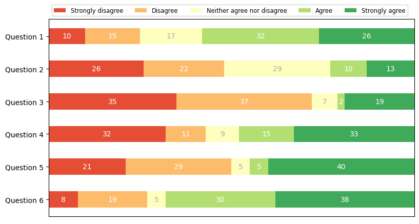
import numpy as np
import matplotlib.pyplot as plt


category_names = ['Strongly disagree', 'Disagree',
                  'Neither agree nor disagree', 'Agree', 'Strongly agree']
results = {
    'Question 1': [10, 15, 17, 32, 26],
    'Question 2': [26, 22, 29, 10, 13],
    'Question 3': [35, 37, 7, 2, 19],
    'Question 4': [32, 11, 9, 15, 33],
    'Question 5': [21, 29, 5, 5, 40],
    'Question 6': [8, 19, 5, 30, 38]
}


def survey(results, category_names):
    """
    Parameters
    ----------
    results : dict
        A mapping from question labels to a list of answers per category.
        It is assumed all lists contain the same number of entries and that
        it matches the length of *category_names*.
    category_names : list of str
        The category labels.
    """
    labels = list(results.keys())
    data = np.array(list(results.values()))
    data_cum = data.cumsum(axis=1)
    category_colors = plt.colormaps['RdYlGn'](
        np.linspace(0.15, 0.85, data.shape[1]))

    fig, ax = plt.subplots(figsize=(9.2, 5))
    ax.invert_yaxis()
    ax.xaxis.set_visible(False)
    ax.set_xlim(0, np.sum(data, axis=1).max())

    for i, (colname, color) in enumerate(zip(category_names, category_colors)):
        widths = data[:, i]
        starts = data_cum[:, i] - widths
        rects = ax.barh(labels, widths, left=starts, height=0.5,
                        label=colname, color=color)

        r, g, b, _ = color
        text_color = 'white' if r * g * b < 0.5 else 'darkgrey'
        ax.bar_label(rects, label_type='center', color=text_color)
    ax.legend(ncol=len(category_names), bbox_to_anchor=(0, 1),
              loc='lower left', fontsize='small')

    return fig, ax


survey(results, category_names)
plt.show()
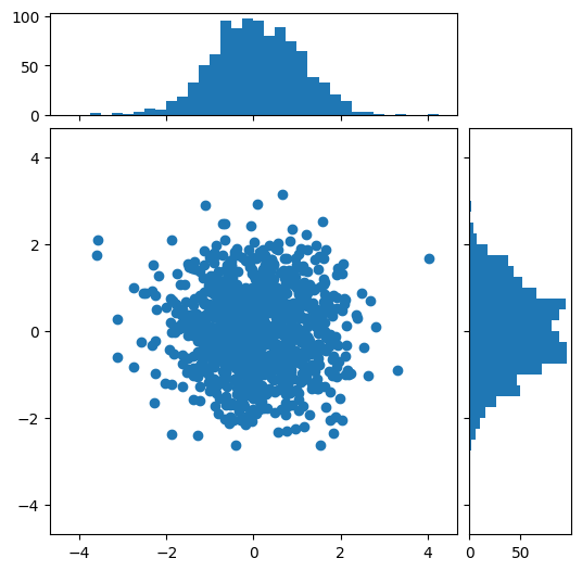
import numpy as np
import matplotlib.pyplot as plt

# Fixing random state for reproducibility
np.random.seed(19680801)

# some random data
x = np.random.randn(1000)
y = np.random.randn(1000)


def scatter_hist(x, y, ax, ax_histx, ax_histy):
    # no labels
    ax_histx.tick_params(axis="x", labelbottom=False)
    ax_histy.tick_params(axis="y", labelleft=False)

    # the scatter plot:
    ax.scatter(x, y)

    # now determine nice limits by hand:
    binwidth = 0.25
    xymax = max(np.max(np.abs(x)), np.max(np.abs(y)))
    lim = (int(xymax/binwidth) + 1) * binwidth

    bins = np.arange(-lim, lim + binwidth, binwidth)
    ax_histx.hist(x, bins=bins)
    ax_histy.hist(y, bins=bins, orientation='horizontal')

# Start with a square Figure.
fig = plt.figure(figsize=(6, 6))
# Add a gridspec with two rows and two columns and a ratio of 1 to 4 between
# the size of the marginal axes and the main axes in both directions.
# Also adjust the subplot parameters for a square plot.
gs = fig.add_gridspec(2, 2,  width_ratios=(4, 1), height_ratios=(1, 4),
                      left=0.1, right=0.9, bottom=0.1, top=0.9,
                      wspace=0.05, hspace=0.05)
# Create the Axes.
ax = fig.add_subplot(gs[1, 0])
ax_histx = fig.add_subplot(gs[0, 0], sharex=ax)
ax_histy = fig.add_subplot(gs[1, 1], sharey=ax)
# Draw the scatter plot and marginals.
scatter_hist(x, y, ax, ax_histx, ax_histy)
Seaborn#
!pip install seaborn
Collecting seaborn
  Downloading seaborn-0.12.2-py3-none-any.whl (293 kB)
     |████████████████████████████████| 293 kB 3.0 MB/s eta 0:00:01
?25hRequirement already satisfied: numpy!=1.24.0,>=1.17 in /home/lyubolp/.local/lib/python3.8/site-packages (from seaborn) (1.24.1)
Requirement already satisfied: matplotlib!=3.6.1,>=3.1 in /home/lyubolp/.local/lib/python3.8/site-packages (from seaborn) (3.6.3)
Requirement already satisfied: pandas>=0.25 in /home/lyubolp/.local/lib/python3.8/site-packages (from seaborn) (1.5.2)
Requirement already satisfied: contourpy>=1.0.1 in /home/lyubolp/.local/lib/python3.8/site-packages (from matplotlib!=3.6.1,>=3.1->seaborn) (1.0.7)
Requirement already satisfied: fonttools>=4.22.0 in /home/lyubolp/.local/lib/python3.8/site-packages (from matplotlib!=3.6.1,>=3.1->seaborn) (4.38.0)
Requirement already satisfied: pyparsing>=2.2.1 in /home/lyubolp/.local/lib/python3.8/site-packages (from matplotlib!=3.6.1,>=3.1->seaborn) (3.0.9)
Requirement already satisfied: packaging>=20.0 in /home/lyubolp/.local/lib/python3.8/site-packages (from matplotlib!=3.6.1,>=3.1->seaborn) (22.0)
Requirement already satisfied: kiwisolver>=1.0.1 in /home/lyubolp/.local/lib/python3.8/site-packages (from matplotlib!=3.6.1,>=3.1->seaborn) (1.4.4)
Requirement already satisfied: python-dateutil>=2.7 in /home/lyubolp/.local/lib/python3.8/site-packages (from matplotlib!=3.6.1,>=3.1->seaborn) (2.8.2)
Requirement already satisfied: pillow>=6.2.0 in /home/lyubolp/.local/lib/python3.8/site-packages (from matplotlib!=3.6.1,>=3.1->seaborn) (9.4.0)
Requirement already satisfied: cycler>=0.10 in /home/lyubolp/.local/lib/python3.8/site-packages (from matplotlib!=3.6.1,>=3.1->seaborn) (0.11.0)
Requirement already satisfied: pytz>=2020.1 in /home/lyubolp/.local/lib/python3.8/site-packages (from pandas>=0.25->seaborn) (2022.7.1)
Requirement already satisfied: six>=1.5 in /usr/lib/python3/dist-packages (from python-dateutil>=2.7->matplotlib!=3.6.1,>=3.1->seaborn) (1.14.0)
Installing collected packages: seaborn
Successfully installed seaborn-0.12.2
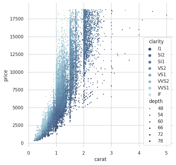
import seaborn as sns
import matplotlib.pyplot as plt
sns.set_theme(style="whitegrid")

# Load the example diamonds dataset
diamonds = sns.load_dataset("diamonds")

# Draw a scatter plot while assigning point colors and sizes to different
# variables in the dataset
f, ax = plt.subplots(figsize=(6.5, 6.5))
sns.despine(f, left=True, bottom=True)
clarity_ranking = ["I1", "SI2", "SI1", "VS2", "VS1", "VVS2", "VVS1", "IF"]
sns.scatterplot(x="carat", y="price",
                hue="clarity", size="depth",
                palette="ch:r=-.2,d=.3_r",
                hue_order=clarity_ranking,
                sizes=(1, 8), linewidth=0,
                data=diamonds, ax=ax)
<AxesSubplot: xlabel='carat', ylabel='price'>
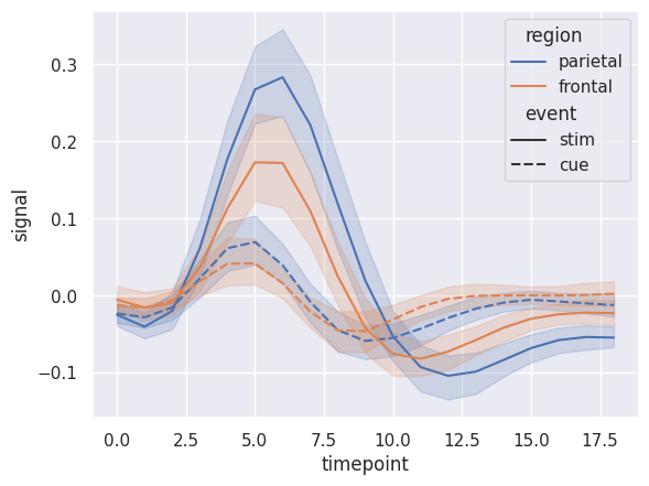
import seaborn as sns
sns.set_theme(style="darkgrid")

# Load an example dataset with long-form data
fmri = sns.load_dataset("fmri")

# Plot the responses for different events and regions
sns.lineplot(x="timepoint", y="signal",
             hue="region", style="event",
             data=fmri)
<AxesSubplot: xlabel='timepoint', ylabel='signal'>
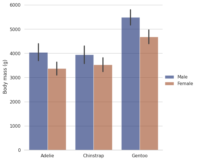
import seaborn as sns
sns.set_theme(style="whitegrid")

penguins = sns.load_dataset("penguins")

# Draw a nested barplot by species and sex
g = sns.catplot(
    data=penguins, kind="bar",
    x="species", y="body_mass_g", hue="sex",
    errorbar="sd", palette="dark", alpha=.6, height=6
)
g.despine(left=True)
g.set_axis_labels("", "Body mass (g)")
g.legend.set_title("")
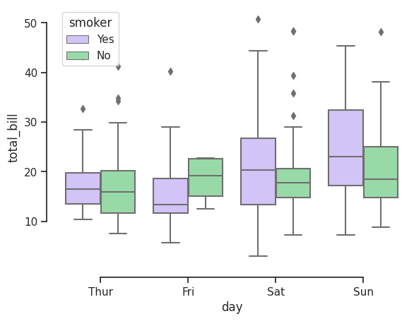
import seaborn as sns
sns.set_theme(style="ticks", palette="pastel")

# Load the example tips dataset
tips = sns.load_dataset("tips")

# Draw a nested boxplot to show bills by day and time
sns.boxplot(x="day", y="total_bill",
            hue="smoker", palette=["m", "g"],
            data=tips)
sns.despine(offset=10, trim=True)
Exploritory Data Analysis#
Ще направим анализ на Titanic dataset-а, с помощта на pandas и matplotlib.